Rating Curves
Welcome to Part 2 in our four-part series of articles about rating curves:
- Rating Curves Part 1: Webinar recording and background resources
- Rating Curves Part 2: What is a rating curve?
- Rating Curves Part 3: Extracting flow and stage results from a 2D model
- Rating Curves Part 4: Sensitivity analyses
What is a rating curve and how do i make one?
As stated in the introduction in Part 1, a rating curve typically correlates water surface elevations with discharge rates. This animation shows two time series hydrographs on the same plot, one with discharge on the primary vertical axis, and one with stage or elevation on the secondary vertical axis:
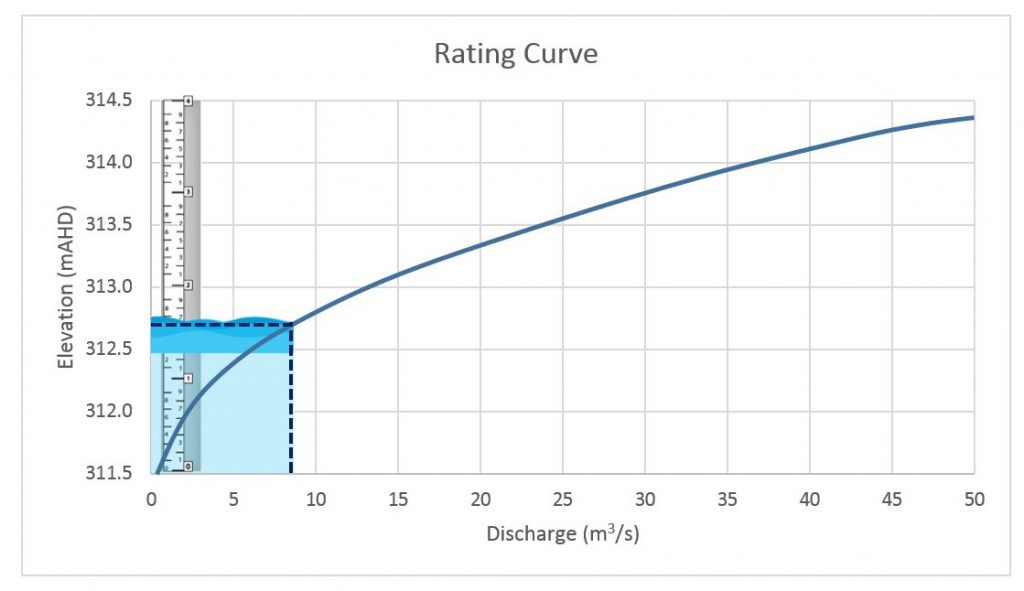
In order to generate a rating curve, we’re essentially taking these two time series hydrographs, removing time as a parameter, and plotting them against each other. In the end, we’re looking for a graphical or tabular representation of the relationship between stage and discharge as shown here:
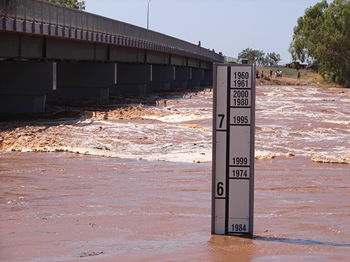
You may run across some rating curves that have the axes reversed, but I prefer to keep stage on the vertical axis since I find it simpler to picture the water surface rising and falling at a gauge like you can see in this animation:
This one shows a very simple case in which the stage-discharge relationship follows a single, smooth path…which is rarely the case in real practice! There are plenty of detailed publications about the complexities of rating curves, so there’s no need to restate all of the theoretical background here. Here are the topics we’ll address in this series of articles, with a focus on extracting and refining rating curves in 1D and 2D hydraulic models:
- Definitions
- Looping or hysteresis
- Differences between rating curves in steady flow and unsteady flow models
- Interpreting rating curves that have been extracted from model results
- Differences between rating curves in 1D and 2D models
- Using 2D models to optimise gauging locations
- Setting up sensitivity runs to estimate confidence levels for rating curve data
- Calibrating hydraulic models to measured gauging station observations
- Using hydraulic models to interpolate and extrapolate rating curve data from measured calibration points
We’ll briefly address generating rating curves from measured data and trying to improve the accuracy of the collected data, but those topics are covered much more comprehensively in the resources we have highlighted in Part 1.
Definition of a rating curve
Most hydrologists understand the term “rating curve” to apply strictly to the relationship between stage and discharge; however, some models like HEC-RAS take a wider interpretation of the term. When you click on the “View Computed Rating Curves” icon in HEC-RAS, for example, it will default to stage versus flow, but the chart can be customised to plot any single variable along the horizontal axis against any number of variables along the vertical axis.
If you click on the “Plot Stage and Flow Hydrographs” icon, however, you’ll see a tab called “Rating Curve” that is limited to stage vs. flow only; for the purposes of this article, we’ll do the same and limit our discussion of rating curves to stage-flow relationships only.
out of time
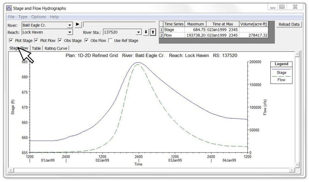
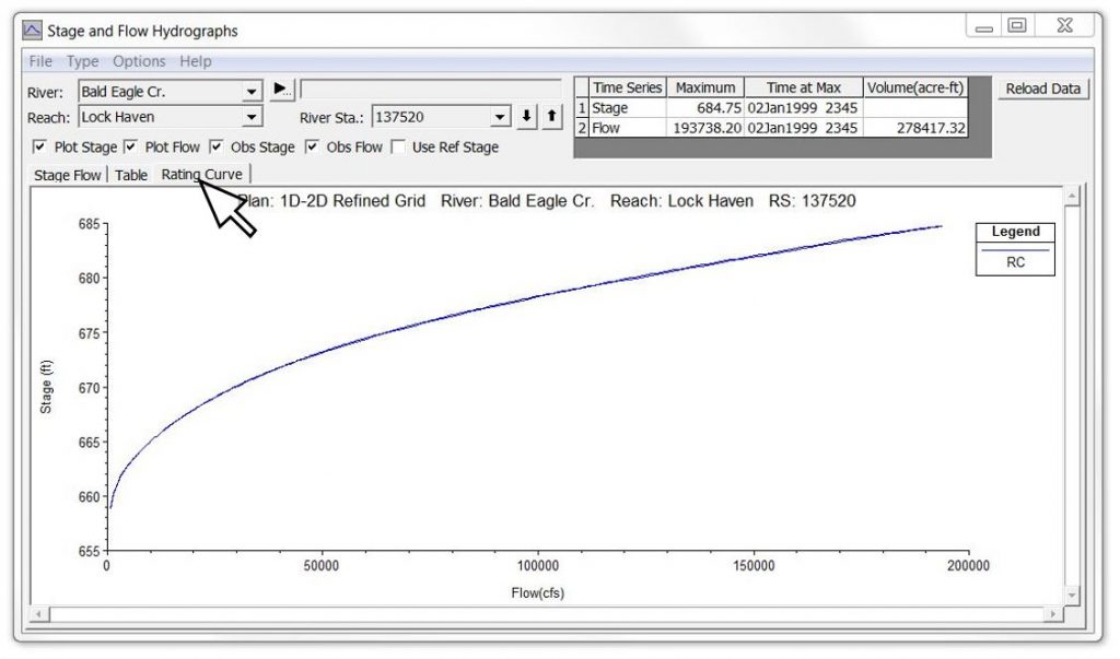
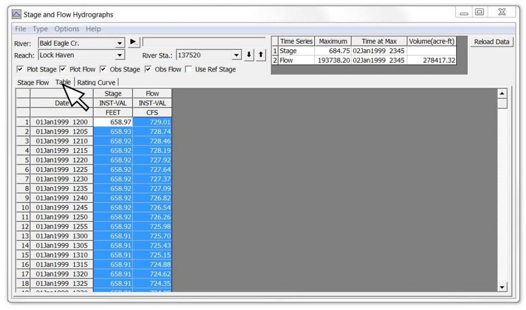
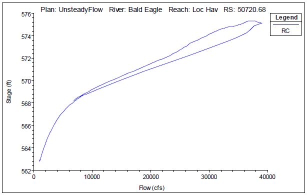
Below is an example of the output options available from the “Plot Stage and Flow Hydrographs” button on the main HEC-RAS command window. This example is from the Bald Eagle Creek example data set that comes with the software and is also included in the HEC-RAS manuals. You can click on the Stage-Flow tab, the Table tab or the Rating Curve tab to see the same data in different ways. This is similar to the combined plot in the first animation above.
The data in the Table tab can be selected, copied, and pasted into Excel or other spreadsheet/plotting program. The other two tabs show the stage and flow data graphically. Because this particular example is from an unsteady flow run, there will be some looping – although in this case it is almost indiscernible unless you zoom in. The “View Computed Rating Curve” icon in HEC-RAS provides essentially the same data but as a single valued rating curve.
We’ll get to the looping effects below, but first let’s cover how we read these curves. If there is no significant looping, any given stage will correspond to the same flow rate, regardless whether the stage occurs during the rising or falling limb of the hydrograph. In the figure below, each of the three stages shown in red, green, and purple corresponds to a single point on the rating curve (click to enlarge):
We’re essentially removing the horizontal time axis and plotting the primary and secondary vertical axes against each other by rotating the secondary axis clockwise by 90 degrees:
steady flow vs. unsteady flow rating curves
1D hydraulic models give you the option of using steady flow or unsteady flow, whereas 2D models typically require a hydrograph with a time axis. When you hit “compute” in a 1D steady-state run, the model assumes that the given flow rate has been running at that rate forever and ever – to infinity and beyond! Even a tiny trickle of water will fill every available storage area (whether it’s noise in your terrain, a massive mining pit, or a hypothetical hole that is dug to the other side of the earth) and instantly appear at the downstream end the model, regardless whether there was ever enough water available to do so. If the trickle would take a billion years to actually fill the hole, your model just travelled a billion years into the future the instant you hit “compute.”
Despite these limitations, sometimes steady flow is good enough – when the peak flow actually occurs after all available storage has been filled, for instance (and if all you’re interested in is the instantaneous peak flow conditions rather than how the water actually got there and how it will recede). Steady flows will certainly give you a much cleaner-looking rating curve by automatically pre-filling all storage and yielding the same energy gradient whether the flow is rising or falling. A rating curve developed from a 1D steady-state run will give you a very nice-looking curve that follows the same path on the way up as on the way down. But does that reflect reality? In some cases it’s perfectly adequate, but it might be worth modelling both ways to check.
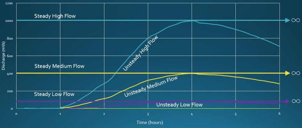
Some 2D models allow you to input a steady flow rate, but this rate is then run over a finite time axis; steady flows aren’t an option at all in HEC-RAS 2D models, for example, unless you generate a flat hydrograph to mimic steady flow conditions. Keep in mind that by generating a flat hydrograph, the volume of water flowing into your system (which can be calculated by integrating the hydrograph and taking the area under the curve) may far exceed any volume that the catchment could possibly deliver – possibly many times greater than the volume of water that could be generated from the PMP rainfall. Remember, a steady flow stays at that rate forever, so the area under that curve is effectively infinite!
Here is an illustration of that concept showing three steady flow rates and three unsteady flow hydrographs that were used for some recent HEC-RAS benchmarking efforts:
If a typical hydrograph is applied to an unsteady flow model (either 1D and 2D), the storage conditions may be different when a particular stage is reached during the rising limb than when that same stage is reached on the falling limb of the hydrograph. In that case, the rating curve will exhibit some form of looping, which is potentially more representative of what actually occurs at most gauging sites.
reading a looped rating curve
Here is an example of a looped rating curve from the same unsteady flow model – this one comes straight out of the HEC-RAS manual:
When looping is involved, the stage-discharge relationship is different during the rising limb of the hydrograph than during the falling limb. The following figure shows one way of using the hydrographs and curves to show the flow rate corresponding to a given stage. The primary and secondary vertical axes have been reversed from the standard plot in HEC-RAS to show the elevation axis in each plot adjacent to each other (click to enlarge):
We’ll dive back into this example in Part 3. Essentially we’ve taken the same steps as above, but this time, the same elevation corresponds to two different flow rates: one on the way up, and the other on the way down.
If you wanted use your unsteady flow hydrograph to generate a single value rating curve with no looping, you could run a set of plan files to represent individual points on the curve. Each flow file would have a single discharge rate that continues for as long as it needs to in order to fill all available storage and reach steady flow conditions where the energy gradient is constant. You could ramp it up the flows by, say, 10 m3/s increments, and run a new plan for each flow rate.
Essentially you have made a pseudo-steady flow file (not to be confused with quasi-unsteady since that’s just for sediment transport in the current version of HEC-RAS). When you record the water surface elevation corresponding to each flow rate, you’ll get a single point on the discharge vs. stage curve. By stitching together a series of points, you could then interpolate values to generate your rating curve.
If you are working with a large number of gauges, this process can be time consuming. Another alternative is to make a composite hydrograph with the time axis stretched out at each flow increment. Instead of a smooth or triangular hydrograph, you might have something like this:
The duration required to reach steady flow conditions at each interval would be different for every system; you may need to stretch each plateau out further than what is shown above. This composite pseudo-steady flow file is basically a series of steady flow rates with a time axis added. Using a hydrograph like the one shown above will generate a choppy rating curve where the flows ramp up, but the points on the curve that represent the steady-state flows will generally form a smooth line representing the steady-state, open channel flow curve.
This approach might be acceptable for systems where flood levels rise and fall slowly, allowing your rating curve to mimic what occurs naturally. If your real floods take five days to pass, for example, but you want to limit your simulation time to a maximum of 24 hours, this can save you some time. In “flashy” systems, however, the flood may arrive so quickly that you may never reach steady conditions. In that case, artificially spreading out the hydrograph can introduce errors, since the looping is a real phenomenon and not just a remnant of the modelling approach.
1d vs. 2d rating curves
In a 1D model, the water surface elevation will be computed and displayed perfectly flat along the entire extent of each cross section. Because the elevation is constant at every point along the section alignment at any given time step, the stage hydrograph will be identical at every point along the line, and a single stage hydrograph can be used to represent the whole section. In 1D, we can thus generate both stage and flow hydrographs for every cross section and easily plot the two parameters against each other; in fact, HEC-RAS will do that for you automatically.
Another inherent constraint of 1D models is that the computed discharge will cross the section line with a flow direction that is exactly perpendicular to its alignment. Even if we’re wrong about the flat water surface or the orientation of the flow as assigned by our selection of the alignment, HEC-RAS will force it to be so in the model.
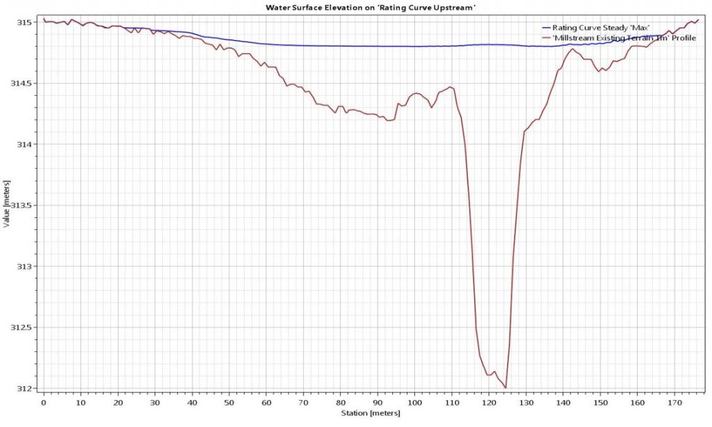
In 2D models, on the other hand, water surface elevations can vary at each computational grid. See the image below for an example of a cross section that has been cut from a 2D model. The water surface elevation varies across the section:
Depending on your mesh resolution, any given cross section could have dozens or even hundreds of different stage hydrographs. To develop a stage-discharge relationship in a 2D model, we therefore need to measure the water surface elevation at the single computational grid element that lies closest to our gauge location.
While stage can be measured at this single point, there can be no flux through a dimensionless point, so we will need to draw a cross section along which to compute discharge. In a 1D model, this will already have been done; for 2D models, however, we do this by defining a profile line. The net flux across the profile line will then be computed based on the resultant velocity vectors for each face point along the profile alignment. We can orient the profile line any way we wish if it passes through the gauge location point and spans the entire wetted channel; the flow direction and the slope of the water surface will be computed independently of the alignment that we select for our profile line.
structure rating curves
Bridges, culverts, and other hydraulic structures have families of rating curves based on inlet/outlet control, orifice vs. weir flow vs. open channel flow, etc.
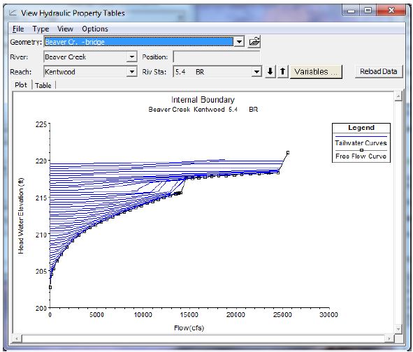
Structures modelled in 1D give you the option of displaying tailwater or backwater curves at each structure. Here is an example of a 1D bridge rating curve from the HEC-RAS manual:
As shown by the tailwater curves, any given stage can correspond to a wide range of discharge rates. Unless you add energy, pressure, or some driving force that affects your energy slope, your upper discharge limit will be the free flow curve. Unless reverse flow is involved, the lower discharge limit for any given stage is zero. In Part 3, we’ll show some examples of negative flows that can just as well correspond to any stage in your rating curve.
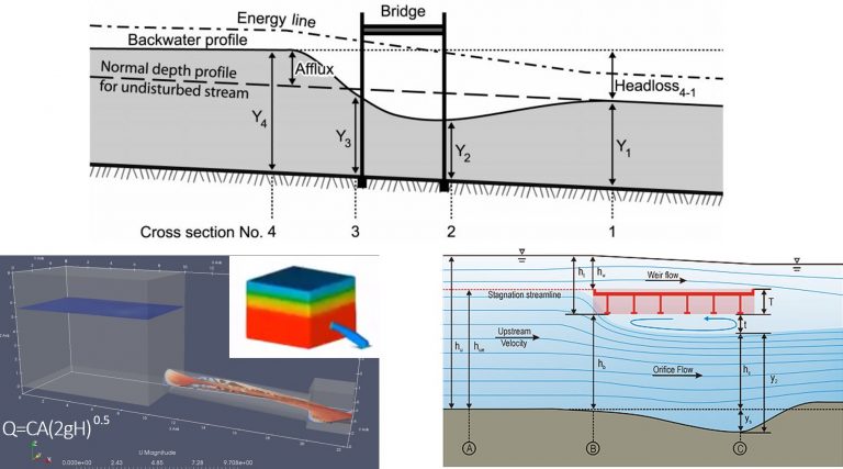
The backwater profile shown in the image below represents flowing water (as indicated by the difference between the energy line and the water surface elevation upstream of the bridge); but a horizontal backwater profile could just as well result from a downstream obstruction that submerges the bridge with no incoming flow at all (in which case the energy line and water surface elevation profile would be coincident).
You can have depth without flow at a given gauging location, but you can’t have flow without depth if that makes sense. That is why a tailwater curve can contain points along the vertical axis, but no points would be plotted along the horizontal axis. If your downstream boundary was a large, static body of water, for instance, you might have a standing water at the structure long after the upstream inflow has receded to nothing. There are plenty of instances in which stream gauges with rating curves that don’t account for tailwater conditions continue to report real-time “flow” when in reality some downstream blockage has simply ponded the water at a still level at the gauge.
The “H” in a typical rating curve for a culvert or bridge is typically the upstream headwater elevation, but the stage in a channel rating curve can be measured wherever the gauge happens to be located. If the stage is measured simply as the water surface elevation without accounting for the velocity head, we could theoretically generate points to the right of the free-flow curve. Take the orifice case shown in the inset above, for instance: if you put a stage gauge in the middle of the jet just downstream of the orifice, it will read a constant elevation regardless of the flow rate. If C, A, and g are held constant in the orifice equation while the “H” in the tank is increased, the discharge through the orifice will increase accordingly. If you plot that rating curve, it will be a horizontal line that could theoretically continue to run to the right of the free flow curve forever while “H” increases. The selected location of the stage gauge is thus critical in providing relevant data for a rating curve as we’ll see in the next articles.
Read the rest of our four-part series of articles on rating curves here, including how to extract rating curves from HEC-RAS and other models:
- Rating Curves Part 1: Webinar recording and background resources
- Rating Curves Part 2: What is a rating curve?
- Rating Curves Part 3: Extracting flow and stage results from a 2D model
- Rating Curves Part 4: Sensitivity analyses

